
HMM for Multidimensional Categorical Data

Are you dealing with sequential data? Do you like classical machine learning? Did you hear about Hidden Markov Model (HMM) but didn’t get a chance to try it on your data? Are you having trouble finding a decent HMM package in Python? If you answered ‘yes’ to at least 1 of the questions above, I invite you to read this article.
I will first explain a bit about HMM model and then present a great Python package with code examples.
Explaining HMM Structure — Using User Behaviour as an Example
HMM is a model that allows you to find the most probable sequence of states, given the data you have (if it is not clear, follow the example). The model is widely used in various domains: sound processing, language models, genetics and many more.
In the following example I will show how HMM was used to predict user behaviour — segments of walking or driving activities. The prediction is based on data from cellular sensors, such as steps counter, GPS locations, WiFi connection etc.
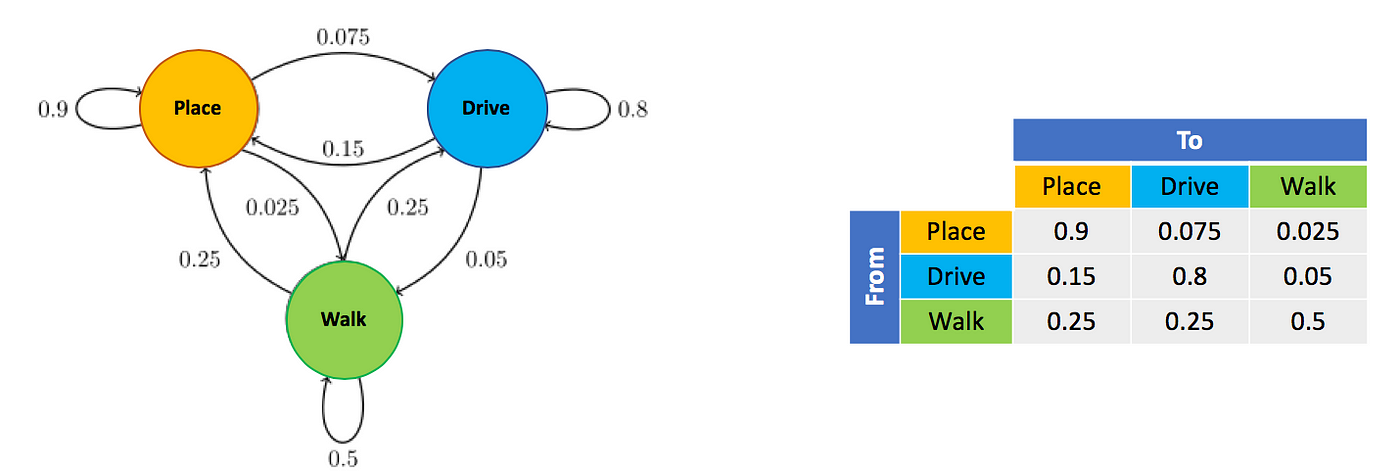
To use a HMM we first need to formalise a statistical model of the world, and all we know about the world will be summarised in 2 small matrices: Transition Matrix and Emission Matrix. Here is a simplified example of how to build these matrices and use them for prediction of user behaviour from cellular sensors:
Let’s assume a user can be in one of 3 states – Driving, Walking or In Place (Place). And let’s assume we have labeled data, where users reported minute by minute what state they were in during the day. For example:
- 08:00 — place
- 08:01 — place
- 08:02— walk
- 08:03 — drive
- etc.
Transition Matrix
A transition probability between state A and state B is the probability that a person, being in state A, will change to state B. We can find the transition probabilities from our labeled data. For example, the transition probability between place and walk will be the number of place minutes followed by walk divided by the total number of place minutes in the data.
We can describe the transition probabilities in one of two ways — a diagram or a Transition Matrix:
Markov Chain
After finding the probabilities, we can build a Markov Chain based on the Transition Matrix.
We will start the chain with one of the events, let’s choose place. Then we will ‘roll a place dice’, meaning we have 90% chance of getting place again, 7.5% chance of getting drive and 2.5% chance of getting walk. Because of the probabilities, we will probably get place again, and we keep rolling the ‘place dice’ until we get to another state, let’s say drive. Then we put the ‘place dice’ aside and use the ‘drive dice’: 80% to continue driving, 15% the get place and 5% to get to walk.
At the end of the day, when we rolled the different dices 1440 times (number of minutes per day) we will get a chain of events:
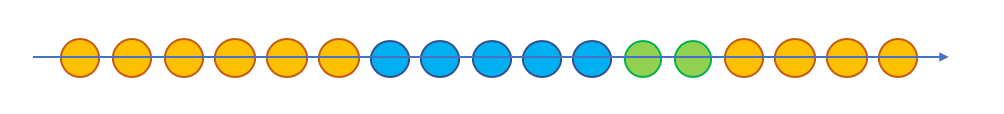
This chain is not yet linked to any information we have from our features (remember we have data from cellular sensors) but it already stores very basic insights about the nature of our data, like the typical duration of each state and the typical sequence of states.
Emission Matrix
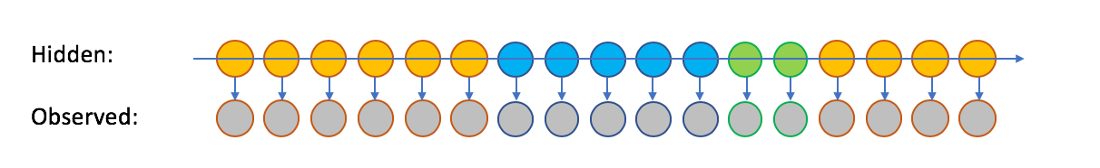
In the world of our problem, the states are hidden and we need to find them based on the observed features, which are the cellphone sensors output (movement, step counter, connection to wifi, etc.).
To include the features in our model we will build the Emission Matrix.
Here is an example of a probability matrix for binary features (features that can only get True/False values) :

The way to build the matrix is also very straight forward — for example, the probability to see wifi connection in place state is the number of minutes with wifi connection while a user was in place state divided by all place state minutes.
Now that we have both transition and emission matrices we can move on to the practical python part!
HMM Python Package
When I embarked on this project, I had a hard time finding a Python package that would be able to work with multidimensional categorical data. I was sure I would find it in my beloved sklearn but I ran into 3 problems:
- The sklearn.hmm module was deprecated a long time ago.
- The GaussianHMM module does support multiple features but doesn’t support categorical features.
- The MultinomialHMM module supports a single categorical feature but doesn’t support multiple features.
So after some Google searching, I found Pomegranate — a great Python HMM package, by Jacob Schreiber. The package is very flexible and easy to use and it supports multiple categorical and continuous features! There are some awesome tutorials on the website, and I would like to present here a small tutorial about how I used it in my case.
Code Examples
(1) Single Dimensional Categorical Data
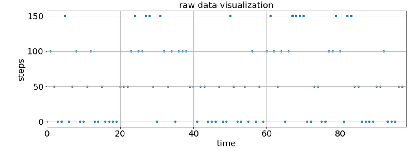
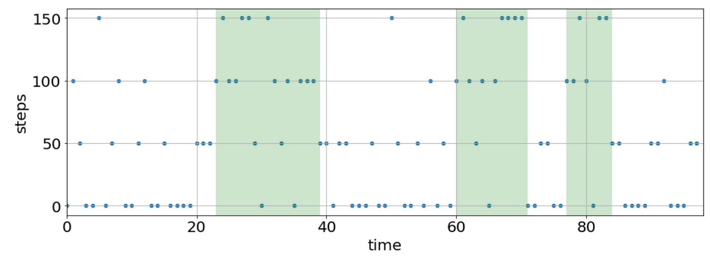
Our data here is a dummy dataset that I created, based on real data. There are 98 minutes and for every minute we have a step counter. I created 4 bins of step counts [0,50,100,150] steps per minute. The goal in this example is to classify the minutes into 2 states: walk and still.
Step 1: Initialise Model & Set Emission Probabilities
Setting the distribution for the steps channel for each state:
- Note: HiddenMarkovModel(), DiscreteDistribution() and State() are all classes of pomegranate package — no need to implement anything 🙂
Step 2: Set Transition Probabilities & Bake Model
Here, I also added start probabilities, which are the probabilities to start the chain from each state.
Visualisation of the Prediction
(2) Multi-Dimensional Categorical Data
Now we can add some complexity and add one more channel to our data (and add as many as we wish later on, using the same code).
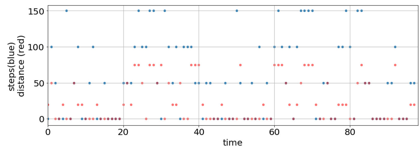
In addition to the step counter, we will add the distance (in meters) of the user’s location between the previous minute and the current one. Let’s break the distances into 4 bins: [0,20,50,75].
Our Data will look like this now:
Step 1: Initialise Model & Set Emission Probabilities
Here we create separate distributions for each feature and each state and then combine the features using IndependentComponentsDistribution.
Step 2: Set Transition Probabilities & Bake Model
Exactly the same…
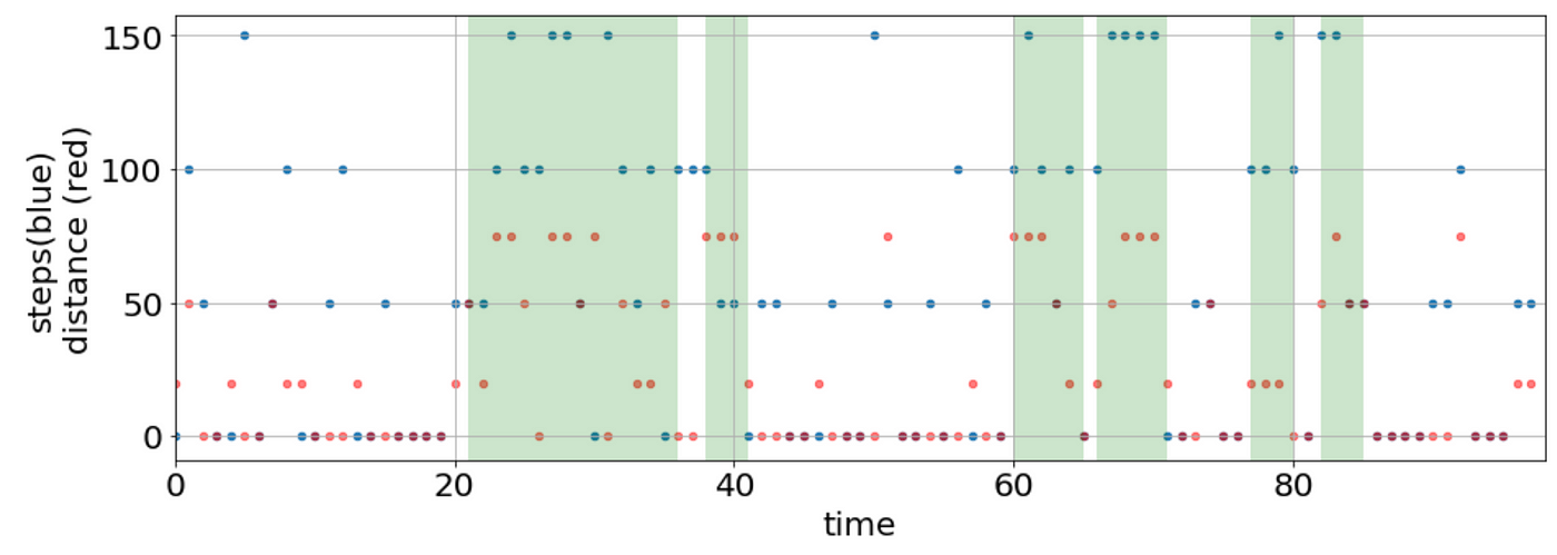
Visualisation of the Prediction
The prediction takes into account data from both features: steps and distance.
Note that we don’t have to bin our data — the package allows us to use continuous distributions like Gaussian distribution. We can even combine discrete distributions for some features and continuous for other features.
I hope you’ve found this post clear and useful and I’d love to hear from your if you have any questions!
I would like to thank
Thanks to Anat Shk, Idit Cohen, Dalya Gartzman, and Lea Cohen

